Theory Guide
- Mohamed Houssem Kasbaoui
Theory Guide
Overview
The equations solved in the CDIFS solver are the constant density incompressible Navier-Stokes equations:
where is the fluid velocity, is pressure, is the sum of the bodyforce (gravity or CPG) and IB forcing. We further assume that the dynamic and kinematic viscosities, i.e., and , are constant.
Spatial Discretization
The governing equations are discretized on a staggered grid with second-order finite-volume schemes.
The variables are staggered as follows:
The figure below illustrates the data layout in a 2D cell
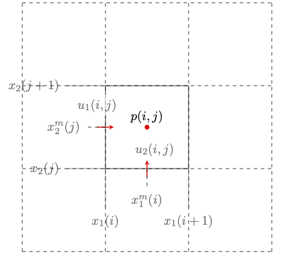
Following the Finite-Volume approach, the discrete quantities , , , and , represent cell averages of the continuous fields:
Note that the integration is carried over a p-cell for , i.e., a cell centered on . Likewise, the integration for velocities is carried over their respective -cells.
The governing equations (1) and (2) are also integrated over the computational cells. Integrating the mass conservation equation (2) over a p-cell and using the divergence theorem gives:
Using the second-order mid-point rule to evaluate the fluxes at the faces
With this, we can define the discrete velocity gradient and divergence operators
Now, let's consider the momentum equation in the -direction. Starting with the pressure gradient,
With this, we define the pressure gradient operator
Computing the pressure gradients in the cell is as follows
Note that the Laplacian operator that appears in the pressure-Poisson equation is built by convolving and operators
Next, we consider the viscous term in the -direction:
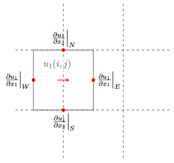
where the gradients on the faces of the -cell are computed with second-order finite-differences:
Thus, we can define the Laplacian operator
Similarly, considering the momentum equation in the -direction gives a second Laplacian
with
Temporal Discretization
The time discretization in CDIFS follows the delta formulation of the Simplified Marker and Cell (SMAC) method with an iterative Crank-Nicolson time scheme. The sequence of operations is as follows
Equation (5) represents the momentum step. Equation (7) is the pressure-Poisson equation. The implicit operator is treated using the approximate factorization:
Thus, equation (5) is solved in three steps
These operations are repeated until . In practice, we use which makes the temporal discretization akin to a second-order Runge-Kutta. Increasing towards approximates a Crank-Nicolson scheme.
Boundary Conditions
When the computational cell is adjacent to a boundary, the operators and ghost cells must be modified to enforce the desired boundary condition. To help with the discussion, we consider that the boundary is on the left-side of the cell . The figure below illustrates the configuration in 2D.
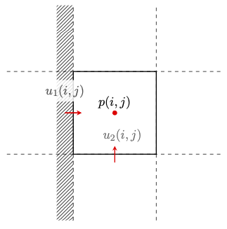
Solid wall
The no-penetration condition at the wall specifies . Unless the wall is static, we may also have tangential displacement: , and . The boundary condition for pressure is 0 gradient in the normal direction . To implement these conditions, we must do the following:
-
Enforce the wall velocity
-
Require that the interpolated tangential velocities at the wall match the boundary conditions
-
Require that in a discrete sense:
-
Require that on the wall, with
-
Require that on the boundary.
Inflow
The treatment for an inflow is nearly identical to the treatment described above. The only difference is that we replace the no-penetration condition with the condition
Outflow
In the case of an outflow boundary, we enforce the Neumann boundary condition
These conditions are implemented in the following way:
-
Require that in a discrete sense:
-
Require that and on the boundary, with
-
Require that on the boundary. For this, we will discretize the gradient with first order lob-sided finite-difference:
-
Require that on the boundary, with
-
Require that on the boundary.